Overview
The anomaly detection (ADM) module consists of three components: on-node anomaly detection (AD), parameter server (PS) and provenance database (ProvDB).
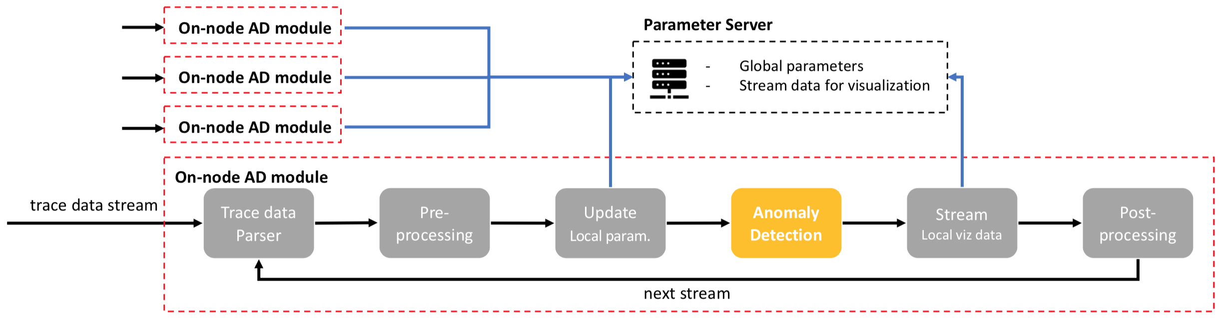
Anomaly detection (AD) module: on-node AD module and paramter server (PS).
As described by the diagram above, an instrumented application communicates trace information to an instance of the AD, whose role it is to decide whether a function execution was anomalous. The decision is based upon globally aggregated function statistics that are collected on the PS and kept in sync with the AD instances. The PS also fulfils the role of collecting global statistics (number of anomalies, various counters) to forward to the external visualization module.
Detailed information about each anomaly is collected by the AD instances and forwarded to the ProvDB, which can be queried both online and offline to obtain more information.
On-node AD Module
The on-node anomaly detection (AD) module (per application process) takes streamed trace data provided by the TAU-instrumented binary. Each AD instance parses the streamed trace data and maintains a function call stack along with any communication events (if available) and counters. The anomaly detection algorithm compares the function execution to those it has seen previously, from which a decision is made as to whether the execution is anomalous. Detailed “provenance” information is collected for every anomaly as well as a limited number of “normal” executions (kept for comparison purposes) and stored in a database. Any remaining trace data is periodically discarded. By focusing primarily on anomalous events, Chimbuko significantly reduces the trace data volume while keeping those events that are important for understanding performance issues.
Below we provide a brief overview of the steps performed by the AD in processing the data.
Parser
Currently, the trace data is streamed from a TAU-instrumented binary via ADIOS2. The streaming is performed in a “stepped” fashion, whereby trace data is collected over some short time period and then communicated to the AD instances, after which the next step begins. We will refer to these steps as “I/O steps” or “I/O frames” throughout this document. We provide a class, ADParser to connect to an ADIOS2 writer side and fetch necessary data for the performance analysis. The parser performs some rudimentary validation on the data, and, depending on the context might augment the data with additional tags; for example, when running a workflow with multiple distinct binaries, the parser appends a ‘program index’ to the data to allow the programs to be differentiated within Chimbuko.
Pre-processing
In the pre-processing step, the AD takes the data for the present I/O step and generates a call stack tree for each program index, rank and thread (See class ADEvent). Communication events, GPU kernel launches and counters that occurred during the function execution are associated with the calls and the inclusive (including child calls) and exclusive (excluding child calls) runtimes are computed.
Anomaly detection
With the preprocessed data the AD instance applies its anomaly detection algorithm to filter the data. In order to provide the most complete and robust information to the algorithm, function execution statistics computed locally are aggregated globally with the data on the Parameter Server (See ADOutlier) prior to performing the anomaly detection.
Anomaly detection algorithm
At present, Chimbuko offers three different algorithms for anomaly detection, that we describe below. All approaches dynamically generate models of the function execution time, which are synchronized through the parameter server. By default the exclusive execution time (excluding child calls) is used but the inclusive time can be used with the appropriate command line option to the AD.
Histogram Based Outlier Score (HBOS) is a deterministic and non-parametric statistical anomaly detection algorithm. HBOS is an unsupervised anomaly detection algorithm which scores data in linear time. It supports dynamic bin widths which ensures long-tail distributions of function executions are captured and global anomalies are detected better. HBOS normalizes the histogram and calculates the anomaly scores by taking inverse of estimated densities of function executions. The score is a multiplication of the inverse of the estimated densities given by the following Equation
\[HBOS_{i} = \log_{2} (1 / density_{i} + \alpha)\]where \(i\) is the index of a particular a function execution and \(density_{i}\) is function execution probability. The offset \(\alpha\) is chosen such that the scores lie in the range \(0\to 100\). HBOS works in \(O(nlogn)\) using dynamic bin-width or in linear time \(O(n)\) using fixed bin width. After scoring, the top 1% of scores are filtered as anomalous function executions. This filter value can be set at runtime to adjust the density of detected anomalies.
This algorithm is quite robust and is able to cope with functions of arbitrary distribution, although the lack of foreknowledge of the appropriate bin width and data range for any given function makes it somewhat susceptible to “compression artefacts” early in the run, although the effects of these can be expected to diminish with time as the model settles and the true peaks become dominant. We recommend this algorithm as the primary, default option.
Sample Standard Deviation (SSTD) defines anomalous function calls as those that have a longer (or shorter) execution time than a upper (or a lower) threshold. The thresholds are defined as follows:
\[\begin{split}threshold_{upper} = \mu_{i} + \alpha * \sigma_{i} \\ threshold_{lower} = \mu_{i} - \alpha * \sigma_{i}\end{split}\]
where \(\mu_{i}\) and \(\sigma_{i}\) are the mean and standard deviation of the execution time of a function \(i\), respectively, and \(\alpha\) is a control parameter (smaller values increase the number of anomalies detected while potentially increasing the number of false-positives).
This algorithm is very simple and its results easy to interpret, but it is susceptible to the poisoning of the model by extreme anomalous events, which when included in the model dramatically increase the standard deviation to the point that no further anomalies are detected. Also, this model implicitly assumes a unimodal distribution of approximately normal distribution, and as such does not adequately describe functions with varying runtimes (perhaps due to being run with different parameters) whose distributions are multimodal.
COPula based Outlier Detection (COPOD) is a deterministic, parameter-free anomaly detection algorithm. It computes empirical copulas for each sample in the dataset. A copula defines the dependence structure between random variables. For this single-dimensional dataset it is equivalent to the cumulative distribution function of the sample distribution. For each sample in the dataset, the COPOD algorithm computes left-tail empirical copula from the left-tail empirical cumulative distribution function, the right-tail copula from the right-tail empirical cumulative distribution function, and a skewness-corrected empirical copula using a skewness coefficient calculated from left-tail and right-tail empirical cumulative distribution functions. These three computed values are interpreted as left-tail, right-tail, and skewness-corrected probabilities, respectively. The lowest probability value results in largest negative-log value, which is the score assigned to the sample in the dataset. Samples with the highest scores in the dataset are tagged as anomalous.
This approach is also histogram-based under-the-hood, but the use of the copula makes it less susceptible to artefacts introduced by the binning procedure. However this algorithm also suffers from an assumption of unimodal data; only data points far above or far below all peaks of the histogram will be labeled as outliers, and those in-between peaks will not.
(See ADOutlier and RunStats, HbosParam and CopodParam).
Provenance data collection
Once anomalous and non-anomalous functions are tagged, Chimbuko walks the call stack and generates detailed provenance information of the anomalous executions and a select number of normal executions (for comparison). (See ADAnomalyProvenance) These data are sent to the centralized “provenance database” for later analysis.
Stream local vizualisation data
The visualization module displays various real-time statistics such as the number of anomalies per rank. This information is collected by the AD (cf. ADLocalFuncStatistics and ADLocalCounterStatistics) and is aggregated on the parameter server, from which it is sent periodically (via curl) to the visualization module. The visualization module is capable also of interacting with the provenance database to obtain detailed information on specific anomalies per user request.
Post-processing
Once the data have been processed the call stack for the present I/O step is discarded and Chimbuko moves onto processing the next step. In this way the amount of trace data maintained is dramatically reduced to just the provenance data and any statistics that we maintain.
Parameter Server
The parameter server (PS) provides two services:
Maintain global anomaly algorithm parameters to provide consistent and robust anomaly detection power over the on-node AD modules.
Keep a global view of workflow-level performance trace analysis results which is streamed to the visualization server and also stored in the provenance database.
Design
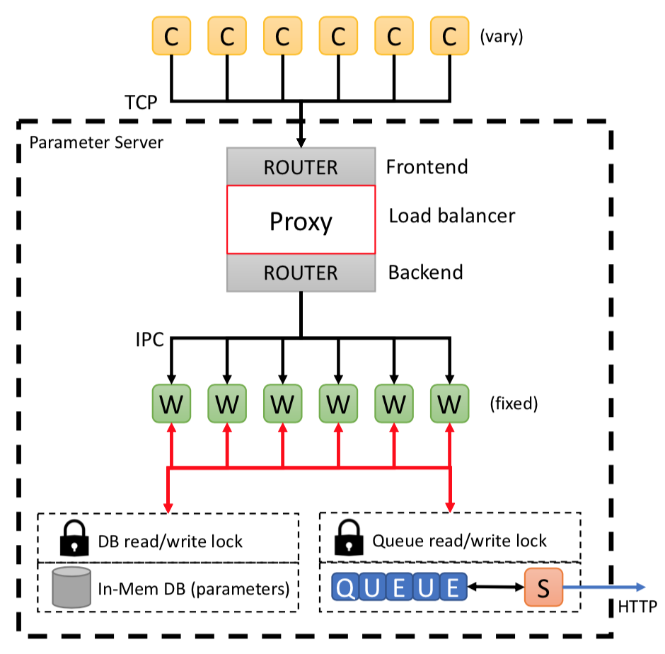
Parameter server architecture
(C)lients (i.e. on-node AD modules) send requests with their locally-computed anomaly detection algorithm parameters to be aggregated with the global parameters and the updated parameters returned to the client. Network communication is performed using the ZeroMQ library and using Cereal for data serialization.
For handling requests from a large number of connected clients the parameter server uses a ROUTER-DEALER pattern whereby requests are sent to a Frontend router and distributed over thread (W)orkers via the Backend router in round-robin fashion.
For the task of updating parameters, scalability is ensured by having each worker write to a separate parameter object in the In-Mem DB. These are periodically aggregated by a background thread and the global model updated, typically once per second such that the AD instances receive the most up-to-date model as possible. Global statistics on anomalies and counters are compiled in a similar way using the data sent from the AD instances (cf. global_anomaly_stats and global_counter_stats) and also stored in this database.
A dedicated (S)treaming thread (cf. PSstatSender) is maintained that periodically sends the latest global statistics to the visualization server.
Anomaly ranking metrics
Two metrics are developed that are assigned to each outlier that allow the user to focus on the subset of anomalies that are most important:
The anomaly score reflects how unlikely an anomaly is. The interpretation is algorithm-dependent but generally a larger number indicates a lower likelihood.
The anomaly severity reflects how important the anomaly is to the runtime of the application. Currently we base this off of the exclusive runtime of the function execution, in microseconds.
The PS includes these values in the provenance information and allows for the convenient sorting and filtering of the anomalies in post-analysis. We are working to present these metrics directly in the online visualization module.
Provenance Database
The role of the provenance database is four-fold:
To store detailed information about anomalous function executions and also, for comparison, samples of normal executions. Stored in the anomaly database.
To store a wealth of metadata regarding the characteristics of the devices upon which the application is running. Stored in the anomaly database.
To store globally-aggregated function profile data and counter averages that reflect the overall running of the application. Stored in the global database.
To store the final AD model for each function. Stored in the global database.
The databases are implemented using Sonata which implements a remote database built on top of UnQLite, a server-less JSON document store database. Sonata is capable of furnishing many clients and allows for arbitrarily complex document retrieval via jx9 queries.
In order to improve parallelizability the anomaly database, which stores the provenance data and metadata collected from the AD instances, is sharded (split over multiple independent instances), with the AD instances assigned to a shared in a round-robin fashion based on their rank index. The database shared are organized into three collections:
anomalies : the anomalous function executions
normalexecs : the samples of normal function executions
metadata : the metadata describing the machine/devices
The global database exists as a single shard, and is written to at the very end of the run by the parameter server, which maintains the globally-aggregated statistics. This database comprises two collections:
func_stats : function profile information including statistics (mean, std. dev., etc) on the inclusive and exclusive runtimes as well as the number and frequency of anomalues.
counter_stats : averages of various counters collected over the run.
ad_model : the final AD model for each function.
The schemata for the contents of both database components are described here: Provenance Database Schema